Sample size for usability study. Part 1. About Nielsen and probability.

In the industry, the number 5 has long been the standard number of users for usability studies.

Google search results for “how many users do you need for usability testing” look like a silent “holy war”:

• Why You Only Need to Test with 5 Users
• 5 users is not enough
• 5 Users Are Enough“…for what, exactly?
• Why 5 is the magic number for UX usability testing
• Why five users are not really enough
• Usability Testing: Why 5 Users Are Enough

And the keynote of each article is the name — Jakob Nielsen.

He is considered to be the main popularizer of the idea, that 5 users are enough for detecting about 85% of interface problems.

In the articles of some authors, Nielsen personifies the dragon, whom they as heroes must defeat, exposing his ideas as a myth. Others, by contrast, talk about his work as one of the most influential in the UX area. Still, a great number of people take the position — “It depends …”.

In this part, I suggest to figure out for ourselves where the idea about “sufficiency of 5 users” came from, what is behind it and how to understand it.

Subject

The rule associated with Nielsen sounds like — 5 users are enough to uncover about 85% usability problems. But such formulation loses sight of the fact, that this phrase is formula-based:

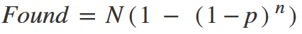
It means — if the interface contains N problems, and the average probability of detecting a problem during one test is λ, then the number of problems, that occurred at least once during the testing of i users will be Found.

From the rule.

The proportion of the found problems (Found) to the total number (N) is our 85%.

i — number of users, 5

But λ — the average probability of detecting a problem in one trial, is not taken into account. Under the initial conditions, which are described above, the value of λ will be 0.31 or 31%.

So we can rephrase the rule: if the proportion of usability problems discovered while testing a single user will be around 31%, then 5 users will be enough to find about 85% of interface problems.

Let’s call it — the 5 users rule.

Background

At the end of each scientific publication, there is a section of references to literature. Because the formation of a theory is usually preceded by a study of other works. And the 5 user rule is not exception.

If you want to learn more about the key historical moments in the formation of the “5 Users” conception, I highly recommend to read the Jeff Sauro’s article A Brief History of the Magic number 5 in usability testing, but I will briefly focus on three authors.

Jim Lewis

In 1982, he published a work, where he discussed how the frequency of occurrence of a problem determines the number of necessary tests to detect it. He proposes to use a binomial distribution to describe this problem, but this topic is touched upon in passing, and the author does not give any formulas.

In 1994, as part of a study, he tested office applications with 15 users. Then, by using the Monte Carlo method, it simulates 500 different user groups. And he compares the research data with data obtained by using a formula based on binomial distribution :

As a result, it concludes, that the experimental and calculated data are consistent.

Robert Virzi

In the late 80s and early 90s, he published several works on the topic of determining the sample size for usability studies. He becomes one of the first, who, based on empirical data, came to the conclusion, that the formula

can be used to predict the proportion of detected problems, depending on the sample size.

After analyzing the data of his study, Virzi draws 3 conclusions:

• 4–5 users are enough to identify 80% of the problems.
• Each subsequent test detects fewer unknown problems.
• The most serious problems are identified by the first users.

Jakob Nielsen

Since the end of the 80s, he has been developed the idea of ​​Discount Usability — lo-fi prototypes, heuristics, iterative design, etc. And as a continuation of this topic, Nielsen and colleagues became interested in determining the minimum number of users that are enough for detecting most interface problems.

Laundaure and Nielsen published a paper in 1993, where they mentioned a formula for determining the number of problems, that can be detected during a usability test.

According to the authors, the formula is based on the Poisson model.

Also, according to the results of the experiments, Laundaure and Nielsen say, that the average probability of detecting problems in one test will be around 30%.

Formula

In the last section, I mentioned two formulas. One is based on the Poisson model, the other one — on a binomial distribution.

Poisson model

Comes from Nielsen & Landauer (1993) study.

we can expect a Poisson model to describe the finding of usability problems (Nielsen & Laundauer, 1993)

But, unfortunately, they do not demonstrate how this formula was derived.

Lewis (2009) also mentioned a conversation with Laundauer, where he said, that the formula is based on:

the constant probability path independent Poisson process model

I also did not find an explanation of why Nielsen & Laundauer refer to this particular type of distribution.

One way or another, the Poisson distribution is associated with continuous events [26], such as time or area. If we are talking about the probability of a call to the support center per unit of time, this is Poisson. But we are talking about the number of events in a certain number of trials, and this is a binomial distribution[22].

Yes, sometimes the Poisson distribution becomes a special case of the binomial distribution. [21] But in this case, the number of trials should be very large, and the probability of an occurring event is very small. What is hard to imagine in the frame of usability study.

So I didn’t find answers. Therefore, let’s note, that there is a way to derive the formula through the Poisson Process.

Binomial distribution

This type of distribution is mentioned in the Lewis (1982, 1994) and Virzi (1990, 1992).

Lewis (1994) explained the principle of deriving the formula:

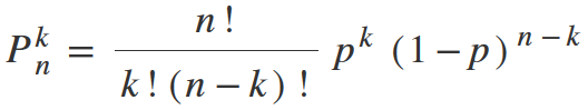
The probability of getting exactly k successes in n independent Bernoulli trials is given by the probability mass function:

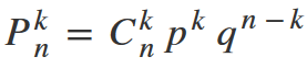
Where,

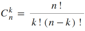
C (k/n) is the number of combinations of test outcomes, for which this event occurs k times in n independent trials. It is calculated by the formula:

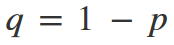
p is probability of event success in one trial.

and q is the probability, that the event we are interested in will not occur. In our case, these p and q probabilities will be the opposite each other, which means:

Let’s rephrase this form in terms of usability researchers.

If the problem detection probability (p) is same for all trials, then the probability P(k /n), that the problem will be detected k times during testing involving n users, will be equal to (finally substituting all other values):

But you should not be afraid, we will simplify everything soon.

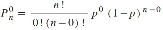
Let’s try to determine the probability, that during the study we will not find any problems, it means a situation, where k = 0

Any number in degree 0 is 1. 0! is also equal to 1. We get:

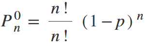
Shorten n! and get the final formula.

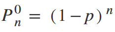
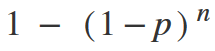
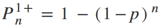
From this formula, it is now easy to get the probability of detecting at least one problem. Again, since the detection of at least one problem and the detection of none problems are opposite events, their sum will be equal to 1, which means:

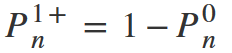
Or:

Important. Each distribution has conditions of use. And binomial distribution is no exception. To apply this formula, the following conditions must be met:

• random sampling
• independent observations
• two mutually exclusive and comprehensive categories of events
• the probability of an event occurring throughout all observations should not change.

Lewis (1994) said that, in general, the usability testing format meets these requirements:

• Although a truly random sample is rarely found in usability studies, nevertheless, moderators do not selectively choose respondents, so the sample can be considered as quasirandom.
• Observations are independent since testing is conducted with each respondent individually. And the problems, that one participant encountered, cannot affect the other.
• Two mutually exclusive and comprehensive categories of problem detection are: the respondent encountered a problem and the respondent completed the scenario without problems.
• In probability theory, this is illustrated by a basket of balls. Let’s imagine — there are 10 balls in a basket, 3 of which are white and 7 are black. Chance to pull out a white ball is 3/10. Let’s suppose, that we get the ball in the first test and it turns out to be white. If we do not return it to the basket, then the probability of pulling out a white ball in subsequent tests will change and will be 2/9. But in the case of usability testing, problems are not “pulled out of the basket” and the probability of a single problem in subsequent tests does not depend on how many users encountered it in previous tests.

The relationship between Lewis-Virzi and Nielsen & Laundaure formulas

As you already noticed, the formulas of Lewis-Virzi and Nielsen & Laundaure are similar. The classical definition of probability will help us to explain their relationship.

The probability of an event is the ratio of the number of cases favorable to it (m), to the number of all cases (n) possible when nothing leads us to expect that any one of these cases should occur more than any other, which renders them, for us, equally possible. [25]

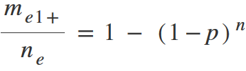
If we speak in the frame of formula based on the binomial distribution. The probability of detecting a problem during testing at least once will be:

Now let’s think about the classical definition for this case.

m — positive outcomes, in our case, this is the number of detected problems.

n — the total number of elementary events, in our case, this is the number of all problems in the interface.

substitute this ratio into the Lewis-Virzi formula:

Multiply both parts of this formula by the total number of problems. We shorten them on the left side and it turns to:

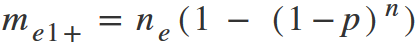
Now back to the Nielsen formula (Nielsen and Laundaure, 1993).

We got 2 identical formulas.

Don’t be misled by the fact, that in one case λ is used, and in the other — p. Within the frame of this formula, both designations are identical. This point is explained in the publication Nielsen (2006):

Nielsen and Landauer used lambda rather than p, but the two concepts are essentially equivalent. In the literature, λ (lambda), L, and p are commonly used to represent the average likelihood of problem discovery. Throughout this article, we will use p.

Therefore, you can write the formula in the form:

In the future, I will not separate Lewis-Virzi and Nielsen formulas.

In general, this formula does not claim any uniqueness. It will be difficult to find at least one textbook on probability theory, wherever this formula is mentioned in the section on multiplying probabilities. [27]

Probability of occurrence of at least one of the independent events A1, A2, …, An, is equal to the difference between the 1 and the multiplication of the probabilities of opposite events.

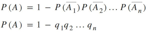
For us, A1, A2, … An are events of detecting a problem during the testing of the first, second … n-th user.

If events A1, A2, …, An have the same probability, what is mean that the probability of detecting a problem remains the same from test to test, then the formula takes a simple form:

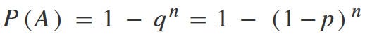
Voila!

The meaning of the 5 users rule

Let’s try to estimate the probability of getting a problem at least once during the study by using the values ​​from the 5 users rule: the probability of a certain problem during the testing of one user is p = 0.31, the number of tests is n = 5.

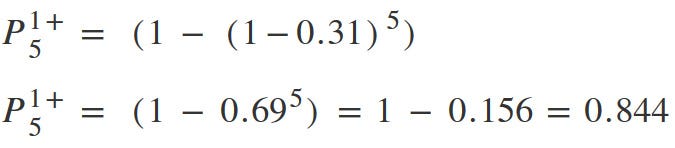
We can say, that during testing by 5 users, with a probability of 85%, we will see a problem at least once, the probability of detection of which in one test will be 0.31.

To simplify the understanding of this calculation, let’s use simple 6-side dices.

Let’s imagine, that we have an event (let’s name it A), whose probability of detection in one test will be the same as in our rule — p = 0.31, which is approximately 2/6.

It means, that our event happens when we rolled 2 of 6 faces. Let’s think it will be 5 and 6.

To demonstrate testing involving 5 users, we need 5 dices.

Throw dices:

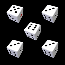
We see, that during testing A event happened 2 times. Good result, but one experiment is not enough, let’s experiment, for example, 20 times.

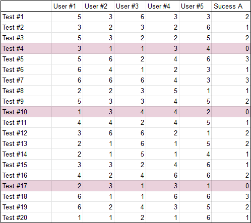
We see, that our event occurred in 17 of 20 tests. So, we get P = 0.85. You can try it yourself.

During a test with 5 users probability of getting a problem at least once will be 85%. But now we are talking about one event — one problem, but in 5 users rule, we make an assumption about all problems.

Let’s use the dices again. But this time, let’s simulate the whole experiment with just one dice. We know now, that in 85% of cases 5 users will face a problem with 0.31 discovery rate.

85% is approximately 5/6

So let’s imagine that any side of dice except 1 is a successful result of the event. But now the event means that 5 users were able to find an issue.

We believe, that in each experiment we can detect any number of problems. So, if we have 6 problems in the interface, the probability of finding wich in a single test is 0.31, then to simulate such an experiment, we just need to throw 6 dices.

And now we see, that testing 5 users will find 5 of 6 interface issues.

If 20 — the same: throw 20 cubes

We will find 17 problems.

If 100. … but I think you understand the principle. Hence the well known — 5 users find 85% of all problems.

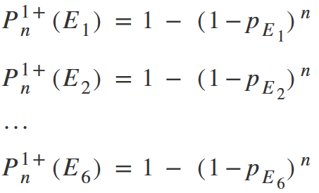
But in reality, all problems are different. This means that the probability of detecting problems in a single test may differ. If, for example, we have 6 problems in the interface, then in the general case we will have 6 formulas:

But in 5 users rule, an assumption is made, based on one formula and the average value of p. To understand how to interpret the result in this case, let’s go back to the previous example.

Add two more events to event A:

event B — with success when we get faces 2,3 or 4

event C — face 1 has fallen.

Thus, we get 3 events, the probability of occurrence of which in individual trials will differ:

event A — 0.3

event B — 0.5

event C — 0.17

Let’s look at our experiment again:

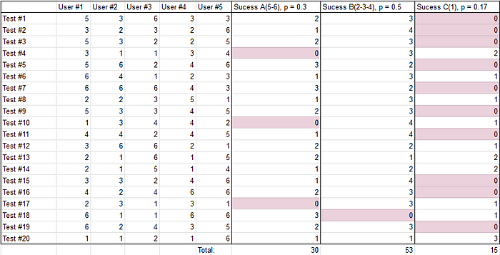
There are two points, which I would like to draw your attention to.

The higher is the probability of an event in a single trial, the more users encounter it. This is a classic definition of probability.

We have 100 elementary events — 20 tests of 5 users.

Event A happened 30 times — 30/100 = 0.3

Event B happened 53 times — 53/100 = 0.53

Event C happened 15 times — 15/100 = 0.15

Probability is not some abstract accident. If we say, that the probability of detecting a problem in one trial will be 0.3, then this means, that 30% of users encounter this problem while interacting with the interface.

Second moment. Let’s look at the probability of an event, occurring at least once as a result of the whole test.

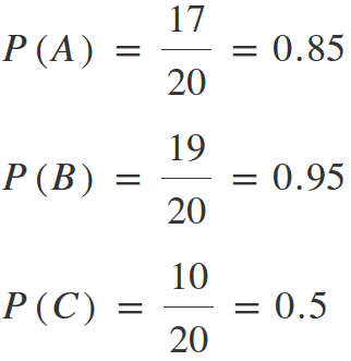
It means, during testing with 5 users in 95% of cases we will encounter problems, that have detection rates equal to 0.5. And only in 50% of cases will we encounter problems with p = 0.17.

Therefore, when we talk about detecting 85% of all problems according to the test results, we mean only problems, the probability of detecting which in a single test will be equal or higher than 0.31.

But don’t get me wrong. I’m not saying that testing 5 users will not reveal rare issues, but in a separate test, we don’t have any significant confidence in this.

This is also confirmed by Jeff Sauro in the article Why you only need to test with five users

So if you plan on testing with five users, know that you’re not likely to see most problems, you are just likely to see most problems that affect 31% -100% of users for this population and set of tasks.

Usage

Now let’s figure out how to use the formula.

To begin with, I recall, that the formula from Nielsen requires knowledge of the total number of problems in the interface.

But if we know how many issues we have, then we probably know what they are. So there is no point in testing. Composing of approximate values ​​is fraught with uncertainty in the results. Therefore, I propose to dwell on a simpler version to use — formula Lewis-Virzi:

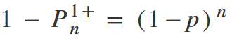
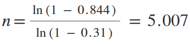
Let me remind you, that we gathered here to calculate the size of the required sample. So, we need to deduce n from this formula.

Let’s move 1 to the left side and multiply by -1 to get rid of the minus in front of the brackets.

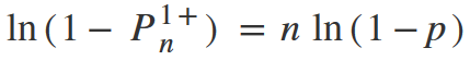
To get rid of the degree, we need to logarithm both parts of the equation.

From here n is equal to:

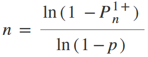
Checking by substituting our calculated values:

But here arises another questions. Where can we get these probabilities?

Choosing P

0.844 is the probability of detecting a problem at least 1 time during testing. If you want more confidence in achieving the problem, please increase this probability. But remember, the higher the probability you put, the more users you will need. Lewis (1994) made a tablet, which is showing the dependence of the number of samples on p and P:

columns 0.01–0.75 is p, the probability of detecting problems while a single user testing

lines 0.04–0.99 — this is P, the probability of detecting a problem at least once according to the results of the whole test

If for some reason you are interested in the repeatability of testing, then you should strive for the highest possible probability of obtaining these results.

Gábor J.Székely gave a good example in his book [28]:

Consider two random events with probabilities of 99% and 99.99%, respectively. One could say that the two probabilities are nearly the same, both events are almost sure to occur. Nevertheless, the difference may become significant in certain cases. Consider, for instance, independent events which may occur on any day of the year with probability p = 99 %; then the probability that it will occur every day of the year is less than P=3%, while if p=99.99% then P=97%.

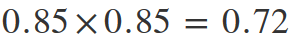
This is the usual multiplication of probabilities. In the example, Székely multiplied 0.99 by itself 365 times. Well, or just raised to a power. As a result, he got a probability equal to 0.026.

Therefore, if the probability of achieving a result during testing is 0.85, and you want to get similar results during the next test, then the probability of such an event will be:

But if the probability of achieving the result will be 0.95, then the probability of achieving a similar result during the next test will be:

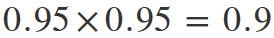
The main thing here is not to use 100% in the formula, otherwise, you’ll get infinity.

Choosing p

As for the average probability of detecting a problem during one testing, there are two ways. Complicated, with questionable accuracy, and simple, but based on an assumption.

Complicated.

To do this, we shave to perform the test on a small sample, for example, on 3 users. Based on the results, we will find a certain number of problems and will be able to calculate the probability of detecting each of the problems in one test. And from here we can calculate the average probability.

For example, we conducted a test and found 10 problems, while each of the users encountered such difficulties:

For this example, we get the average probability of detecting a problem during one test 0.53.

To understand why this approach is questionable, look again at the tablet, that I made, based on the Lewis (1994).

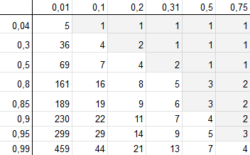
With gray, I have noted cases for 3 users sample. So, with 95% confidence, we can be sure, that we will find a problem, the probability of getting which in one test is p = 0.75. But if we are talking about p = 0.31 problems, then there is already the probability of detecting at least one such problem while testing on 3 users will be 50%, which is already not so good. But we may have also much more rare problems.

Simple.

Jeff Sauro in one of his articles suggested not guessing and producing uncertainties. Simply choose the minimum probability of problems, that you want to detect during the test. For example, you can say, that for us enough to detect problems, that affect 50% of users — p = 0.5 or you may want to detect problems, that affect even 1% of your users, then p = 0.01.

That’s all folks. Now we can substitute the chosen values ​​and calculate the sample.

Conclusion

Taking into account all of the above, we can rephrase 5 users rule so that it would more correspond to reality:

If during testing, the experiments are independent, and the sample is at least quasirandom, then we can assume, that with 5 users testing, we will find 85% of the problems, encountered by at least 31% of users.

But it is too early to put an endpoint here. We have not considered any critic publications yet. So, to be continued.

References

Publications

• Bevan, N., Barnum, C., Cockton, G., Nielsen, J., Spool, J., Wixon, D. (2003). The “magic number 5”: Is it enough for web testing?. CHI Extended Abstracts. 698–699.
• Caulton, D. (2001). Relaxing the homogeneity assumption in usability testing. Behaviour & Information Technology, 20(1), 1–7.
• Cazañas-Gordón, A. & Miguel, A. & Parra Mora, E. (2017). Estimating Sample Size for Usability Testing. ENFOQUE UTE. 8. 172–185.
• Crouch, M., & McKenzie, H. (2006). The logic of small samples in interview-based qualitative research. Social Science Information, 45(4), 18.
• Faulkner, L. (2003). Beyond the five-user assumption: Benefits of increased sample sizes in usability testing. Behavior Research Methods, Instruments, & Computers 35: 379
• Fusch, P. I., & Ness, L. R. (2015). Are we there yet? Data saturation in qualitative research. The Qualitative Report, 20(9), 1408–1416.
• Grosvenor, L. (1999).Software usability: Challenging the myths and assumptions in an emerging field. Unpublished master’s thesis, University of Texas, Austin.
• Guest, G., Bunce, A., & Johnson, L. (2006). How many interviews are enough? An experiment with data saturation and variability. Field Methods, 18(1), 24.
• Henstam, P. (2018) How many participants areneeded when usabilitytesting physical products?
• Katz, Michael & Rohrer, Christian. (2004). How Many Users Are Really Enough…And More Importantly When?
• Kessner, M., Wood, J., Dillon, R., West, R. (2001). On the reliability of usability testing.
• Lewis, J. (1982) Testing Small System Customer Setup. Proceedings of the Human Factors Society 26th Annual Meeting p. 718–720
• [13] Lewis, J. (1994). Sample Sizes for Usability Studies: Additional Considerations. Human factors. 36.
• Lewis, J. (2009). Evaluation of Procedures for Adjusting Problem-Discovery Rates Estimated From Small Samples. International Journal of Human–Computer Interaction
• Molich, R., Bevan, N., Curson, I., Butler, S., Kindlund, E., Miller, D., Kirakowski, J. (1998). Comparative evaluation ofusability tests. In Proceedings of the Usability Professionals Association (pp. 189–200). Washington, DC: UPA
• Nielsen, J. and Molich, R. (1990). Heuristic evaluation of user interfaces. In Proc ACM CHI’90.
• Nielsen, J., Landauer, T. (1993). A mathematical model of the finding of usability problems. In Proceedings of the INTERACT ’93 and CHI ’93 Conference on Human Factors in Computing Systems (CHI ‘93). ACM, New York, NY, USA, 206–213
• Nielsen, J., Turner, C., Lewis, J. (2002). Current Issues in the Determination of Usability Test Sample Size: How Many Users is Enough?
• Nielsen, J., Turner, C., Lewis, J. (2006). Determining Usability Test Sample Size.
• Sauro J. (2008). Deriving a Problem Discovery Sample Size
• Spool, J., Schroeder, W. (2001). Testing Web Sites: Five Users Is Nowhere Near Enough.
• Thomson, Stanley. (2011). Sample Size and Grounded Theory. JOAAG. 5
• Vasileiou, K., Barnett, J., Thorpe, S. et al. (2018). Characterising and justifying sample size sufficiency in interview-based studies: systematic analysis of qualitative health research over a 15-year period. BMC Med Res Methodol 18, 148
• Virzi, R. A. (1990). Streamlining the design process: Running fewer subjects. Proceedings of the Human Factors Society 34th Annual Meeting p. 291–294
• Virzi, R. A. (1992). Refining the test phase of usability evaluation: how many subjects is enough? Human Factors, 34, 457–468.
• Walker, J. L. (2012). The use of saturation in qualitative research. Canadian Journal of Cardiovascular Nursing, 22(2), 37–46.
• Woolrych, Alan., Gilbert, C. (2001). Why and when five test users aren’t enough.
• Wright, Peter & Monk, Andrew. (1991). A Cost-Effective Evaluation Method for Use by Designers. International Journal of Man-Machine Studies. 35. 891–912. 10.1016/S0020–7373(05)80167–1.

Articles

• [1] A Brief History Of The Magic Number 5 In Usability Testing https://measuringu.com/five-history/
• [2] Filling Up Your Tank, Or How To Justify User Research Sample Size And Data https://www.smashingmagazine.com/2017/03/user-research-sample-size-data/
• [3] Getting Big Ideas Out of Small Numbers https://www.cooper.com/journal/2013/05/getting-big-ideas-out-of-small-research/
• [4] How Many Test Users in a Usability Study? https://www.nngroup.com/articles/how-many-test-users/
• [5] How to Determine the Right Number of Participants for Usability Studies https://www.uxmatters.com/mt/archives/2016/01/how-to-determine-the-right-number-of-participants-for-usability-studies.php
• [6] How Investing in UX Will Save Your Business Money & Time https://www.marketpath.com/blog/investing-in-ux-will-save-business-money-time?fbclid=IwAR0IwK09D1bXQAIKAwBZf8NtJWkX4Ybc4X-FWQxKWJVmXnDrati9kG5llt8
• [7] Jeff Sauro’s thoughts about sample size https://measuringu.com/tag/sample-size/
• [8] Qualitative Sample Size — How Many Participants is Enough?https://www.drjohnlatham.com/many-participants-enough/
• [9] The 5 User Sample Size myth: How many users should you really test your UX with? https://www.experiencedynamics.com/blog/2019/03/5-user-sample-size-myth-how-many-users-should-you-really-test-your-ux
• [10] The Five Most Influential Papers In Usability https://measuringu.com/five-papers/
• [11] What sample size do you really need for UX research? https://www.userzoom.com/blog/what-sample-size-do-you-really-need-for-ux-research/
• [12] Why its bullshit to test with 5 users (unless you are asking the right questions) https://conversionista.com/en/blogg/why-its-bullshit-to-test-with-5-users/
• [13] Why you don’t need a representative sample in your user research https://www.userfocus.co.uk/articles/myth-of-the-representative-sample.html
• [14] User Research: is more the merrier? https://uxdesign.cc/user-research-is-more-the-merrier-9ee4cfe46c7a
• [15] User testing: How many users do you need? https://blog.maze.design/user-testing-how-many-users/
• [16] How many users need for usability test (rus) https://usabilitylab.ru/blog/usability-testing-respondents/

Calculators

• [17] Bernoulli trials table https://planetcalc.com/7044/
• [18] Dice Roller https://www.random.org/dice

About Monte Carlo Methods

• [19] An Overview of Monte Carlo Methods https://towardsdatascience.com/an-overview-of-monte-carlo-methods-675384eb1694
• [20] Accuracy and Efficiency of Monte Carlo Method https://inis.iaea.org/collection/NCLCollectionStore/_Public/19/047/19047359.pdf

Math

• [21] Deriving the Poisson Distribution from the Binomial Distribution https://medium.com/@andrew.chamberlain/deriving-the-poisson-distribution-from-the-binomial-distribution-840cc1668239
• [22] Difference between Poisson and Binomial distributions. https://math.stackexchange.com/questions/1050184/difference-between-poisson-and-binomial-distributions
• [23] Poisson Processes https://images-na.ssl-images-amazon.com/images/G/01/books/stech-ems/Intro-to-Stochastic-Modeling-4E-sample-9780123814166._V154961835_.pdf
• [24] Why Does Zero Factorial Equal One? https://www.thoughtco.com/why-does-zero-factorial-equal-one-3126598
• [25] Classical definition of probability https://en.wikipedia.org/wiki/Classical_definition_of_probability
• [26] Poisson distribution https://en.wikipedia.org/wiki/Poisson_distribution
• [27] Probability of occurrence of “at least one” https://www.teachoo.com/4154/768/Example-14---Probability-of-atleast-one-of-A--B-is-1---P(A-)-P(B-)/category/Examples/
• [28] Székely, G. J. (1986) Paradoxes in Probability Theory and Mathematical Statistics, Reidel.